Biokit is an unified wrapper package for functions and utilities to perform the analysis of transcriptomic and proteomic data. It contains several functions to carry out a basic exploratory analysis of the omics data tables, together with tools to normalize and perform the differential analysis between the sample groups of interest. In addition, biokit can also conduct the functional analysis of the results to reduce its dimensionality and increase its interpretability, using over-representation analysis (ORA) or functional class scoring (FCS) approaches.
Installation
The package can be installed through the install_github() function from devtools.
Case-of-use
library(biokit)
data("sarsCovData")
data("humanHallmarks")

# set output directory for images
knitr::opts_chunk$set(
  fig.path = "man/figures/"
)
To exemplify the capabilities and features of biokit, we will apply it to a transcriptomic dataset obtained from the following GEO entry. This dataset contains a subset of the samples analyzed in this project, where the reaction from different human cell lines to SARS-COV-2 infection is evaluated using RNA-Seq. The starting materials for the analysis are:
The RNA-Seq counts table
head(sarsCovMat[, 1:3])## NHBE_Mock_1 NHBE_Mock_2 NHBE_Mock_3
## DDX11L1 0 0 0
## WASH7P 29 24 23
## FAM138A 0 0 0
## FAM138F 0 0 0
## OR4F5 0 0 0
## LOC729737 112 119 113A data frame containing the sample group information
head(sarsCovSampInfo)## name group
## 1 NHBE_Mock_1 NHBE_Mock
## 2 NHBE_Mock_2 NHBE_Mock
## 3 NHBE_Mock_3 NHBE_Mock
## 4 NHBE_SARS.CoV.2_1 NHBE_SARS.CoV.2
## 5 NHBE_SARS.CoV.2_2 NHBE_SARS.CoV.2
## 6 NHBE_SARS.CoV.2_3 NHBE_SARS.CoV.2And a list containing the MSigDb functional categories, that we will use for the functional analysis
lapply(humanHallmarks[1:10], head)## $HALLMARK_ADIPOGENESIS
## [1] "ABCA1" "ABCB8" "ACAA2" "ACADL" "ACADM" "ACADS"
##
## $HALLMARK_ALLOGRAFT_REJECTION
## [1] "AARS" "ABCE1" "ABI1" "ACHE" "ACVR2A" "AKT1"
##
## $HALLMARK_ANDROGEN_RESPONSE
## [1] "ABCC4" "ABHD2" "ACSL3" "ACTN1" "ADAMTS1" "ADRM1"
##
## $HALLMARK_ANGIOGENESIS
## [1] "APOH" "APP" "CCND2" "COL3A1" "COL5A2" "CXCL6"
##
## $HALLMARK_APICAL_JUNCTION
## [1] "ACTA1" "ACTB" "ACTC1" "ACTG1" "ACTG2" "ACTN1"
##
## $HALLMARK_APICAL_SURFACE
## [1] "ADAM10" "ADIPOR2" "AFAP1L2" "AKAP7" "APP" "ATP6V0A4"
##
## $HALLMARK_APOPTOSIS
## [1] "ADD1" "AIFM3" "ANKH" "ANXA1" "APP" "ATF3"
##
## $HALLMARK_BILE_ACID_METABOLISM
## [1] "ABCA1" "ABCA2" "ABCA3" "ABCA4" "ABCA5" "ABCA6"
##
## $HALLMARK_CHOLESTEROL_HOMEOSTASIS
## [1] "ABCA2" "ACAT2" "ACSS2" "ACTG1" "ADH4" "ALCAM"
##
## $HALLMARK_COAGULATION
## [1] "A2M" "ACOX2" "ADAM9" "ANG" "ANXA1" "APOA1"In a first step, we can explore the per-sample value distribution of the raw counts table. Then, we can filter and normalize the count matrix using a minimum cutoff of counts across samples, with a default value of 15. Then, we can normalize the resulting count matrix with the edgeR TMM approach, using the countsToTmm() function from the biokit.
biokit::violinPlot(sarsCovMat)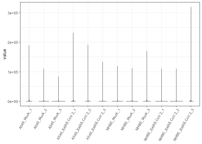
sarsCovMat <- sarsCovMat[rowSums(sarsCovMat) >= 15, ]
tmmMat <- countsToTmm(sarsCovMat)
Next, we can explore the new per-sample value distribution using again the violin plot function.
biokit::violinPlot(tmmMat)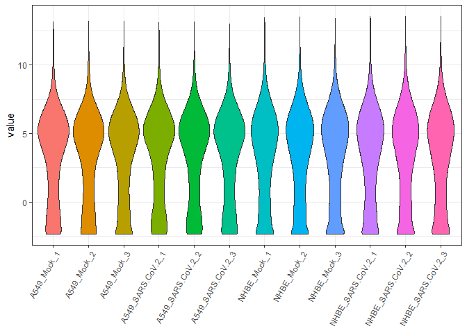
In a second exploratory step, we can apply a Principal Component Analysis (PCA) to reduce the dataset dimensionality and explore the group distribution in a bidimensional space formed by the first two principal components.
biokit::pcaPlot(mat = tmmMat, sampInfo = sarsCovSampInfo, groupCol = "group")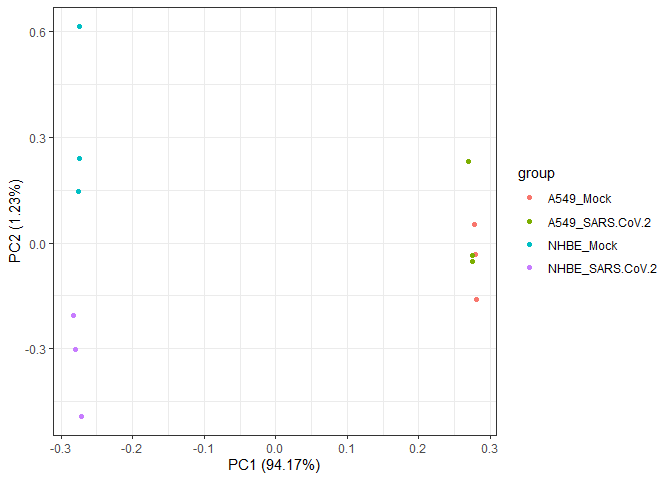
Next, we can explore the top 25 genes with the higuest standard deviation in teh entire dataset, representing and clustering them through a heatmap representation.
heatmapPlot(mat = tmmMat, sampInfo = sarsCovSampInfo, groupCol = "group",scaleBy = "row", nTop = 25)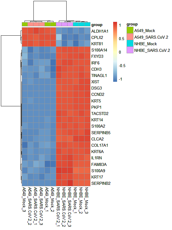
Once that we have evaluated the distribution of sample groups and of most variable genes with basic exploratory analysis, we can perform a differential expression between the sample groups of interest using the for the linear models included in the limma package. The volcanoPlot() function can be used to obtain a broad spectrum view of the results for each of the comparisons carried out.
diffRes <- biokit::autoLimmaComparison(mat = tmmMat, sampInfo = sarsCovSampInfo, groupCol = "group")
biokit::volcanoPlot(diffRes)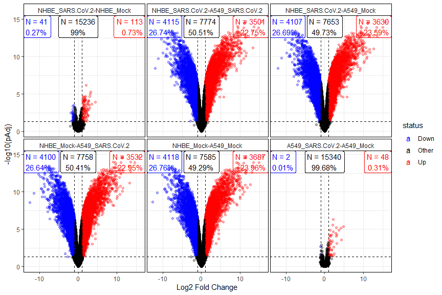
In a final step, we can perform the functional analysis for each comparison using the GSEA approach and visualize the significant results using the gseaPlot() function.
gseaResults <- gseaFromStats(df = diffRes, funCatList = humanHallmarks, rankCol = "logFc", splitCol = "comparison")
gseaPlot(gseaResults)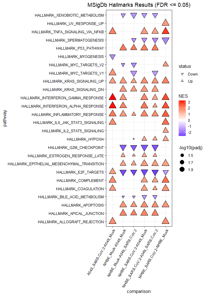
Session information
## R version 4.0.5 (2021-03-31)
## Platform: x86_64-w64-mingw32/x64 (64-bit)
## Running under: Windows 10 x64 (build 19042)
##
## Matrix products: default
##
## locale:
## [1] LC_COLLATE=English_United Kingdom.1252
## [2] LC_CTYPE=English_United Kingdom.1252
## [3] LC_MONETARY=English_United Kingdom.1252
## [4] LC_NUMERIC=C
## [5] LC_TIME=English_United Kingdom.1252
##
## attached base packages:
## [1] stats     graphics  grDevices utils     datasets  methods   base
##
## other attached packages:
## [1] biokit_0.1.1
##
## loaded via a namespace (and not attached):
##  [1] locfit_1.5-9.4              Rcpp_1.0.6
##  [3] lattice_0.20-41             tidyr_1.1.3
##  [5] assertthat_0.2.1            digest_0.6.27
##  [7] utf8_1.2.1                  R6_2.5.0
##  [9] GenomeInfoDb_1.26.4         stats4_4.0.5
## [11] RSQLite_2.2.5               evaluate_0.14
## [13] highr_0.8                   ggplot2_3.3.3
## [15] pillar_1.6.1                zlibbioc_1.36.0
## [17] rlang_0.4.10                data.table_1.14.0
## [19] blob_1.2.1                  S4Vectors_0.28.1
## [21] Matrix_1.3-2                rmarkdown_2.7
## [23] labeling_0.4.2              BiocParallel_1.24.1
## [25] stringr_1.4.0               pheatmap_1.0.12
## [27] RCurl_1.98-1.3              bit_4.0.4
## [29] munsell_0.5.0               fgsea_1.16.0
## [31] DelayedArray_0.16.3         compiler_4.0.5
## [33] xfun_0.22                   pkgconfig_2.0.3
## [35] BiocGenerics_0.36.0         htmltools_0.5.1.1
## [37] tidyselect_1.1.0            SummarizedExperiment_1.20.0
## [39] tibble_3.1.0                gridExtra_2.3
## [41] GenomeInfoDbData_1.2.4      edgeR_3.32.1
## [43] IRanges_2.24.1              matrixStats_0.58.0
## [45] fansi_0.4.2                 crayon_1.4.1
## [47] dplyr_1.0.6                 bitops_1.0-6
## [49] grid_4.0.5                  gtable_0.3.0
## [51] lifecycle_1.0.0             DBI_1.1.1
## [53] magrittr_2.0.1              scales_1.1.1
## [55] stringi_1.5.3               cachem_1.0.4
## [57] farver_2.1.0                XVector_0.30.0
## [59] limma_3.46.0                ggfortify_0.4.11
## [61] ellipsis_0.3.2              generics_0.1.0
## [63] vctrs_0.3.8                 fastmatch_1.1-0
## [65] RColorBrewer_1.1-2          tools_4.0.5
## [67] bit64_4.0.5                 Biobase_2.50.0
## [69] glue_1.4.2                  purrr_0.3.4
## [71] MatrixGenerics_1.2.1        parallel_4.0.5
## [73] fastmap_1.1.0               yaml_2.2.1
## [75] AnnotationDbi_1.52.0        colorspace_2.0-0
## [77] GenomicRanges_1.42.0        memoise_2.0.0
## [79] knitr_1.31
